Excel: How to use the LOOKUP function

Excel is the ideal tool for handling large quantities of data. But creating massive tables in the Microsoft program is rarely intended as an end in itself. You also need to be able to work with the values. If you regularly find yourself spending far too long looking for the correct entries and values, the program can create more problems than it solves. Fortunately, besides formulas for statistics and algebra, Excel offers search and reference functions in its toolbox. In particular, these include the very helpful LOOKUP function.

Let’s imagine you have a table with at least two columns. For each entry in the first column, there’s a corresponding value in the second column in the same row. If you want to find out the value for a certain entry, you can either manually scroll down the rows or you can search for it with the LOOKUP function. Enter the search term into the formula and Excel will give you the relevant value. Alternatively, you can also create a formula with a search field. You can then easily integrate the cell with the search term into the LOOKUP formula.

This direct application of the function is already very useful. But combining LOOKUP with other functions is even more practical. Nesting allows you to either pull the search term from the result of another function or to pass on the found value to another function for further processing.

LOOKUP can be used in two different ways in Excel: as a vector or matrix function. The vector function is probably the most popular variant.

• Search criterion: Here you enter the content you want to search for. Numerical values, text (in quotation marks), logical values, cell references, or another formula can be used in this position.
• Search vector: This term defines in which cells the function should search for the entered criterion. In most cases, you’ll enter a cell range here. But you can also directly input the values in the form of an array (in curly brackets) into the parameter.
• Result vector: The optional parameter for the result vector allows you to set the range in which the corresponding value can be found. It’s therefore important that this parameter is the same size as the search vector – no matter if you enter a cell range or an array. If you don’t complete this parameter, Excel automatically applies the search vector as the result vector.

With the vector variant, you can always only enter a row or column for the search or result range. But the two vectors don’t need to lie directly together. As long as both parameters are the same size, the two ranges can be found in completely different places in the spreadsheet.

The search function is always approximate. This means the search criterion doesn’t have to be an exact match with one of the values in the search vector. Excel will then try to find the next smallest value. But this can only work if you sorted the list in ascending order beforehand. If the table is mixed up, the function will provide incorrect results.

Microsoft advises against using LOOKUP as a matrix function. Instead, VLOOKUP or SLOOKUP should be used for this purpose.

In this case, the function will not only work within a column or row, it will include a larger area (a matrix) in the search.

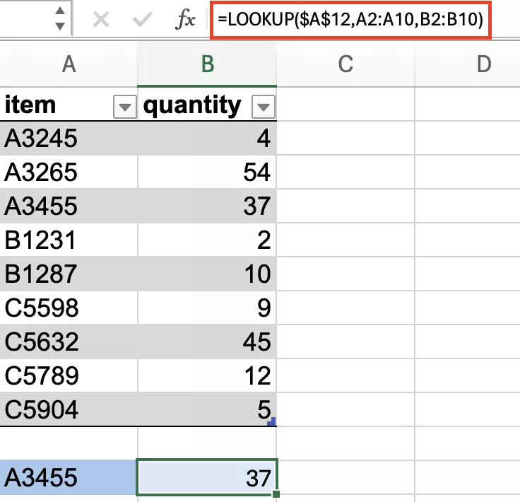
As already mentioned, LOOKUP is easiest to use in the form of a search formula. It enables you to search through an entire column, for example, and find the corresponding value. In our example below, we use an inventory list. Each item group has its own name. We’d like to search for the quantity in stock for each.

Enter the respective inventory number into the search field. The LOOKUP function will then display the number of items. You can now dynamically search for each item number.

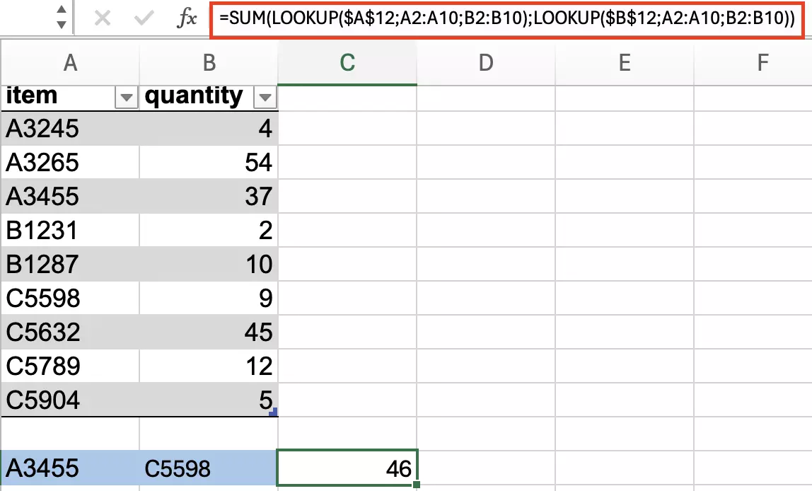
However, the LOOKUP function can also be effectively combined with other Excel functions. For instance, the results of a LOOKUP or multiple LOOKUPs can be added together.

The formula will now add the number of two different items.

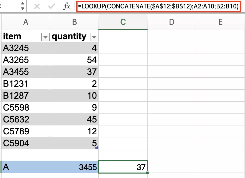
But you can also enter the search criterion using a formula. In our example, the item names always comprise a combination of a letter and a number. You can also enter these two elements separately and then consolidate them with the CONCATENATE function. Since the first part of the names only consist of one of three possible letters, it’s even worth creating a drop-down menu for this purpose.

You can now use two separate search fields to find out the number of an item group.

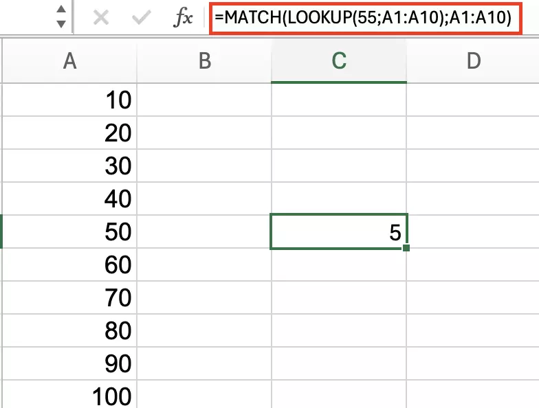
The LOOKUP function has another advantage when using the approximate search and leaving the result vector empty: it allows you to determine which value within a list comes close to the searched value. When you combine this operation with the Excel function MATCH, Excel even shows the row where the value can be found.