

How to create a drop-down list in Excel

Many users don’t use Excel to perform a one-time calculation, but instead use workbooks on a regular basis. In such cases, being able to select certain information directly from a list simplifies and speeds up the process of working with spreadsheets. Here, we run through the steps for how to create a drop-down list in Excel.
The following instructions can be applied to Microsoft 365 as well as Excel versions 2021, 2019 and 2016.
Quick guide for creating an Excel drop-down list
The following quick guide shows you how to create drop-down menus in Excel quickly and easily.
- Fill in a table with the values that you want to appear in the drop-down list. It’s best to create this table on a separate sheet.
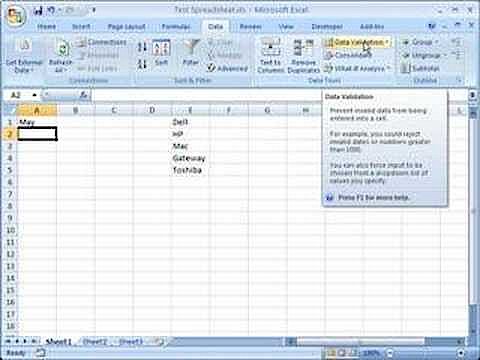
- Select the cell where you want to create the list. Click on the Data tab. In the tools section, click Data Validation.
- In the Allow field, select List and in the Source field, select the table elements you created earlier. Click OK.
Now your Excel drop-down list is ready. Click on the gray box to select an element from the drop-down list.
- Office Online
- OneDrive with 1TB
- 24/7 support
What are drop-down lists in Excel used for?
A drop-down menu enables you and other users to select specific values or information from a list. This provides a number of advantages:
- The different values can be selected with just one click, meaning that you don’t have to type the entire item or number every time.
- Typos are prevented by having users select options from a list.
- Because the values are predefined, other users can’t generate errors by entering incorrect values.
Drop-down lists give you and other users a significantly greater level of convenience, while also making many forms look much more professional.
What you need to know about adding a drop-down list in Excel
A drop-down list is always located in a cell. For this reason, the corresponding cell must be formatted in order to use a drop-down list in Excel. At the same time though, you also need a table with values, which will then be displayed in the drop-down list. It is a good idea to create this on a separate worksheet in the same workbook so that the entries are available at all times but can also be neatly hidden. This list should also be created as an Excel table because Excel can process it better that way, and any changes made to the table are reflected immediately in the linked drop-down list.


In the actual worksheet, select the cell in which you want the drop-down list to appear. Then go to the Data tab in the ribbon. Here you will see the Data Validation item in the tools category. When you click this, a new menu containing the Validation criteria will open. This area gives you the option to allow only whole numbers or text of a specific length, for example.


To add the drop-down list, List needs to be selected. Now specify where the table with the values is located. You can enter this directly, however, because the table is located on another worksheet, you will also have to manually enter this as well. Alternatively, you can use the selection function where you simply highlight the area with the relevant values using the mouse. The information will subsequently appear in the drop-down list.
Make sure that the In-cell drop-down option is enabled, otherwise the list will only be regarded as being there to stop manual entries being made and no drop-down list will be created.


You can now integrate the information from the Excel drop-down list into various functions. For example, the IF function can be used to trigger another calculation or event depending on the selection made.


Want to adapt or change your Excel drop-down list? In our dedicated article, you can find out how to edit drop-down lists in Excel.
 To display this video, third-party cookies are required. You can access and change your cookie settings here.
Reviewer

Jeanna Raffa
With over 18 years of experience in online marketing, Jeanna Raffa possesses extensive expertise in digital marketing. Since 2020, her focus has been on providing practical information regarding email, office, and cloud storage solutions.