How to use the Excel INDIRECT function
When using Excel, we often use cell references in formulas. The INDIRECT function in Excel lets you go one step further. Rather than writing the cell reference in the formula, you can simply obtain it from another cell or put it together based on multiple parameters.
This tutorial can be used with the 2021, 2019 and 2016 versions of Excel.
Quick overview of how to use Excel INDIRECT
- Use the syntax
=INDIRECT(reference). - For the
referenceparameter, you can either specify a cell (e.g.,C2) or write the column and row separately and combine them with an ampersand&(e.g.,C&2) - You can also reference a cell from another worksheet. In the formula
INDIRECT("'"&Worksheet&"'!Cell"), you need to provide the name of the worksheet and the cell containing the value you’re looking for.
What can the INDIRECT Excel function be used for?
With INDIRECT, Excel allows you to obtain a reference from another cell, instead of entering it directly into the formula. Users can also piece together cell references in this manner – extracting the first component from one cell and the second one from another. The cell containing the INDIRECT function then displays the value that the compound reference refers to. INDIRECT is rarely used on its own. However, it could be used in this way for certain dynamic formulas, where the cell reference changes continuously as new parameters are entered in a cell. In most cases, INDIRECT is used in combination with other functions. It’s also possible to use INDIRECT to display a value from another worksheet. In theory, you could even refer to another workbook. But this kind of reference only works when the other workbook is also open. If the file referred to in the INDIRECT function is closed, an error message will appear instead of a value.
With HiDrive cloud storage from IONOS, you can securely save, edit and share your Office documents in one centralized location. Whether for personal or professional use, you can work flexibly from any device with the HiDrive app and other interfaces.
What is the syntax for Excel INDIRECT?
INDIRECT has a mandatory and an optional parameter.
=INDIRECT(ref_text;[A1])- ref_text: This is where you enter the cell reference or cell references. You can also write a part of the cell reference into the formula directly (using quotation marks). Two reference components can be combined with the ampersand character (&).
- A1: This optional parameter specifies the format you wish to create the cell reference in. If the parameter is left out or TRUE is entered in the formula, the A1 format is applied. In the case of FALSE, the formula uses the R1C1 format.
Excel is typically used in A1 format. Here, the rows are numbered (A1, A2, A3, …) and the columns are shown with letters that progress in alphabetical order (A1, B1, C1, …). But you can also configure the program settings if you want to use the R1C1 format. With this format, both rows and columns are numbered. For example, R5C10 would denote the cell where the fifth row meets the tenth column.
The R1C1 notation comes from Multiplan, Excel’s predecessor. You can still activate the reference style today under Formulas in the Options menu.
Examples of how to use INDIRECT in Excel
One way to use the INDIRECT function is to link references together. If the cell A1 contains B1 and the cell B1 contains the value 5, the following formula would produce the value 5:
=INDIRECT(A1)Excel recognizes the text entry in cell A1 as a signal for the cell reference and interprets it accordingly.

The function becomes more complex when the cell reference is split into parts.
=INDIRECT("B" & A1)In this example, instead of entering the entire cell address in A1, only the number component of the cell reference has been entered. The letter in the formula designates the column (in this case “B”). The letter is combined with the value in A1 using the ampersand & to create the cell reference B1.

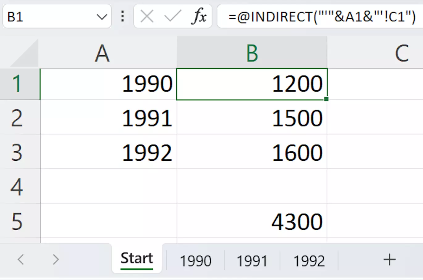
INDIRECT also offers an interesting application when the Excel INDIRECT function is used to reference values in other worksheets. This can be useful, for example, if similar tables and calculations are contained in multiple sheets and you wish to display the selected values of other sheets in an overview sheet. Here, the name of the worksheet is obtained from a cell.
=INDIRECT("'"&A1&"'!C1")Cell A1 contains the name of the worksheet and in that sheet, the desired value is located in cell C1. The additional symbols in the function’s parameter arise from the fact that the full text of the reference (including quotation and exclamation marks) has to be included. For the necessary quotation mark, a single quotation mark needs to be placed within double quotation marks, since it concerns a text entry in the function. The text from cell A1 and subsequently a longer text entry then follows. The worksheet name is closed again with a quotation mark followed by an obligatory exclamation mark and finally the cell with the value you want to display.

You can now adjust the value in cell A1 as needed. You can do this, for example, using a drop-down list. Alternatively, you can arrange the values of the different sheets one below the other. Here you can simply drag down the formula (using the cursor) and Excel will automatically adjust the references to the new position of the function.
How to use the Excel INDIRECT function with other functions in Excel
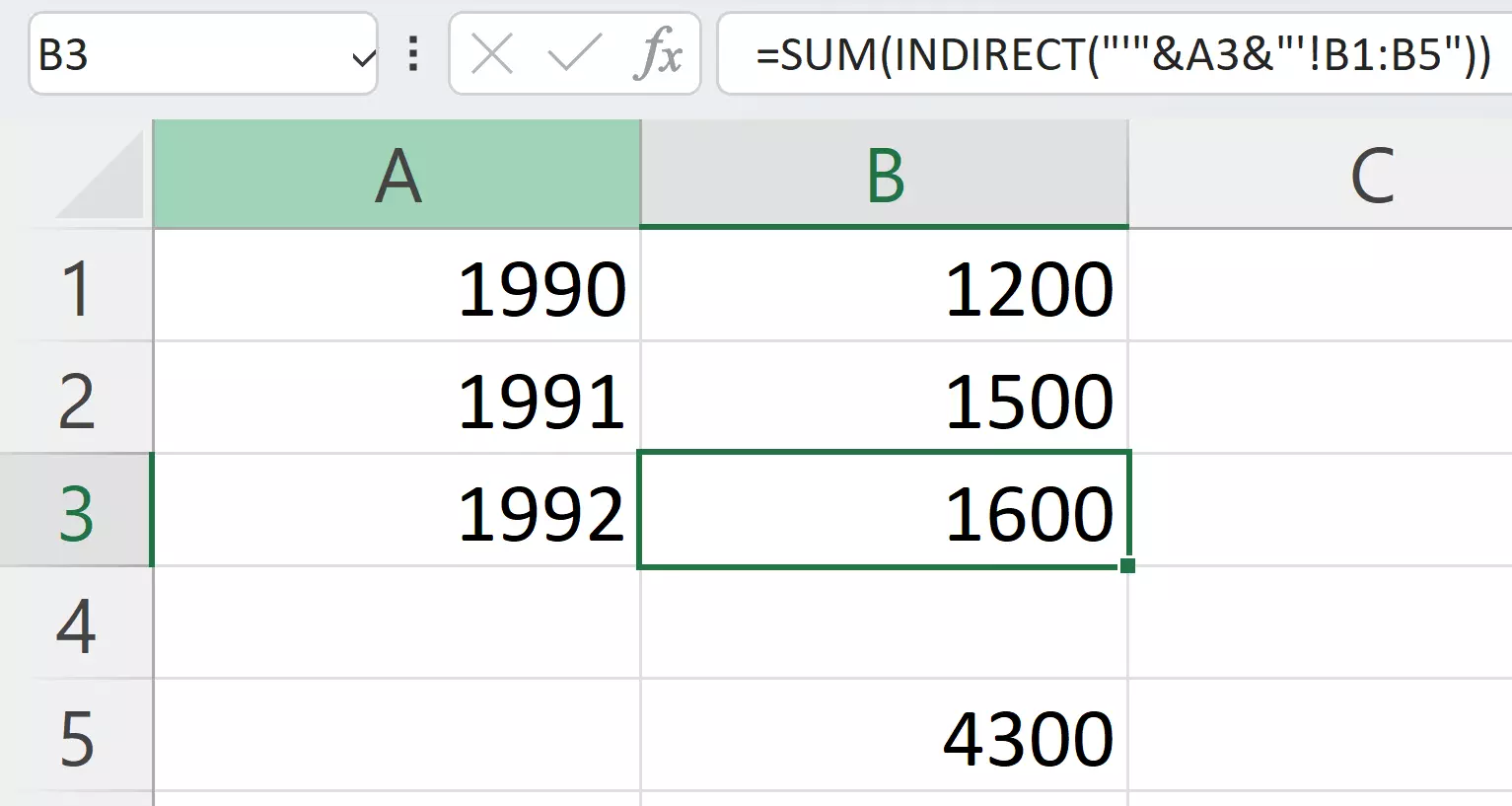
The INDIRECT Excel function is often used in conjunction with others. For example, combining INDIRECT with the SUM function is useful if you want to add values from another worksheet. Rather than generating the total in the corresponding sheet and then reproducing it in an overview, like in the example earlier, the values can be added directly in the overview.
=SUM(INDIRECT("'"&A3&"'!B1:B5"))This formula allows you to add cells B1 to B5 in a worksheet that you have specified in cell A3.

You can also add values from different worksheets with the SUM function.
=SUM(INDIRECT("'"&A1&"'!C1”);INDIRECT("'"&A2&"'!C1”);INDIRECT("'"&A3&"'!C1"))
Many other mathematic or statistical functions (such as MEAN) can also be expanded upon in Excel using this technique.
- Store, share, and edit data easily
- Backed up and highly secure
- Sync with all devices

