Excel MATCH Function Explained
Why Do You Need MATCH in Excel?
In large tables, it can sometimes be complicated to find a specific value. Although Excel, like other Office applications, offers a search function, the result cannot be further processed. If you want to know where a particular element is located in the table and then transfer the result to another formula, you need to use a special Excel function. While the various lookup functions reproduce the contents of a specific cell in the context of the search query, MATCH can specify the position of the cell which contains the search term.
The search result is not output as absolute cell information, but in the form of a relative position: The result always refers to the position of the searched area. You can search within either a column or a row. The search result shows how many values from the left (for a row) or from above (for a column) the search criterion is located.
Excel MATCH: Syntax
The MATCH function has three parameters, with the last being optional.
=MATCH(search criterion; search array; [match type])Meaning of the individual parameters:
- Search criterion: Here you enter the value you are searching for. This can either be a number or text, which you then put in quotation marks.
- Search array: At this point, you enter the cell range to be searched. The from-to area is marked with a colon.
- Match type: This information is optional. This specifies how exactly the search should be performed. The specification -1 finds the smallest value that is greater than or equal to the search criterion; 1 is the largest value that is less than or equal to the search criterion; 0 just searches for an exact match.
If you leave the last item blank, Excel will automatically assume 1. If you choose one of the two match types that do not search for an exact match, the values in the search area must be sorted; ascending for type 1 and descending for type -1.
It is also possible to specify the search array, not in the form of cell references, but to write values directly into the cell. The values are then entered in curly brackets and separated with semicolons.
Excel does not take uppercase and lowercase into account when searching, even if you’re looking for an exact match. In addition, the search criterion does not have to be entered directly in the function. Instead, the term or value to be found may be in another cell which you simply refer to.
Remember that you always start functions in Excel with an equals sign (=). Otherwise, the program recognizes the input as plain text. In addition to entry via the formula bar, you can also use the function assistant. Excel will guide you through inputting the parameters.
MATCH Explained by an Example
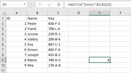
Suppose you have created a table with three columns. In the middle column are names. In this column, you can now search for a specific person by performing an exact search (match type 0) for text (in quotation marks) in the MATCH function.
=MATCH("Simon";B2:B10;0)MATCH Combined with Other Functions
The advantages of the MATCH function arise primarily in combination with other Excel formulas. Nesting allows the result of MATCH to be passed to another function.
Excel: MATCH + VLOOKUP
For example, the interplay between MATCH and VLOOKUP is very successful. The latter function requires the specification of the column index. In VLOOKUP, you must always specify the location of the column in which the result is located. This is where MATCH comes into play: With the MATCH function, the column index does not have to be counted, but can be determined using a search term.
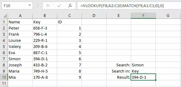
In our example, we want to know which key belongs to Simon. Instead of entering “2” as the column index, MATCH can be used to determine the position. This also allows dynamic formulas to be created. The search criteria are then embedded in the functions via cell references.
=VLOOKUP(F8;A2:C10;MATCH(F9;A1:C1;0);0)The search term is in cell F8 and the column from which the result is to come in F9. For easier handling you can also enter a drop-down list. The MATCH function accesses the search term in F9 and looks for it in the top column. The function passes the result to the VLOOKUP, where it becomes the column index. The advantage: If you want to now find the result in another column, the function adapts dynamically.
Excel: MATCH + INDEX
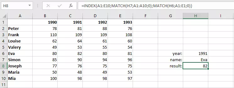
The MATCH function can also be combined very well with the INDEX function. While exploring a simple table by using the VLOOKUP function, you can also use this combination to analyze an array. The INDEX function returns the contents of a cell, and therefore needs a row and a column specification. These determine two nested MATCH functions in the other function. Again, we use cell references so that the settings can be easily changed.
=INDEX(A1:E10;MATCH(H7;A1:A10;0);MATCH(H6;A1:E1;0))The first comparison function provides information on the position of the row, the second one returns the corresponding column. This way, the INDEX function can return the content. Since this is done with a cell reference, you can easily adjust the setting here as well.


